1) Introduction
Should 30-year-old centerbacks be signed for large transfer sums or to 5-year contracts? How about 30-year-old wingers? How much better is a “raw” 21-year-old really going to get? How many seasons of “peak” performance can you expect to get out of a player?
Ultimately, this paper seeks to determine how aging impacts the performance of football players. On the surface, this may not seem to be the most awe inspiring research topic for two reasons: first, the impact of aging is inherently heterogeneous; there is no single aging curve that perfectly characterizes the impact of aging on each individual player. Second, the perceived need for precise research on this topic appears minimal, given that the footballing sphere has already implicitly incorporated an understanding of this topic into their decision-making processes: players in their late teens and early twenties are given time to develop and fetch high transfer fees due to their perceived potential to improve. Conversely, players in their early and mid thirties are rarely given long-term contracts and are unlikely to transfer for large sums of money. This research, though maybe not at the cutting edge of data analytics, aims to precisely quantify how age generally impacts a player’s performance. Further, given the heterogeneous nature of aging, I propose methods to characterize the range of likely aging curves among both individual footballers and individual position groups.
Generally, I find that footballers reach their “peak,” defined as their maximum level of performance, at around 27.4 years of age. In addition, I find that there is significant heterogeneity in the impact of aging on player performance, at both the individual and position level. Specifically, I find that wingers age relatively quickly: wingers tend to peak the youngest, at 26.1 years of age, and decline in ability faster than players in other positions. In contrast, I find that centerbacks age relatively slowly: centerbacks tend to peak around 27.5 years of age and decline in ability slower than players in other positions.
This paper will be structured as follows: first, I will discuss the primary existing methodologies that have been used to assess the impact of aging on athlete performance, along with their methodological limitations. Second, I will introduce how generalized additive models (GAMs) can be used to better understand how aging impacts footballer performance. Third, I will use GAMs, along with a tensor variable, to characterize the heterogeneity in aging curves among football players, thereby, at least partially, addressing the need for individual inquiry. Finally, I will conclude with some of the possible limitations of this research and various high level takeaways.
At this point, I would like to note that this research is an adaptation and extension of CJ Turturo’s Flexible Aging in the NHL Using GAM, which attempted to quantify the impact of aging on professional ice hockey player performance. I am extremely grateful for CJ’s work, which served as an invaluable resource to build off of. Further, I will reference CJ Turturo’s research frequently throughout the remainder of this paper.
2) Aging Curves
Basic Aging Curve
An aging curve is simply a curve constructed by plotting age against an outcome variable, where, presumably, the outcome variable’s relationship with age is of interest. Typically, in the context of evaluating aging on athlete performance, two different types of statistics are used as the “outcome variable”: in some cases, when determining how age impacts specific skills, such as goal scoring, dribbling, or passing, micro statistics are used. In other cases, though, such as this one, more comprehensive statistics that aim to evaluate the total value of a player’s performance, such as wins above replacement (WAR), are used as the outcome variable. Given that football players, across different positions, have vastly different micro statistic profiles, meaning that various micro statistics will not be relevant to an individual’s overall performance, I will be using “Isolated Impact,” a metric explained here that isolates the impact of each individual player on xGF and xGA per 90 minutes, controlling for teammates, opposition, managers, and other variables, as the outcome variable.1 Specifically, I will use a data set containing the Isolated Impact scores for each player in Europe’s top 5 leagues for each season from 2014/15 through 2020/21. For each season, a player’s “age” is defined as their age on August 1, just prior to the start of the season.
\(~\)
| Figure 1: Number of Observations by Age | ||||||
|---|---|---|---|---|---|---|
| Age | Centerback | Fullback | Central Midfielder |
Winger | Striker | Total |
| 15 | 0 | 0 | 4 | 2 | 2 | 8 |
| 16 | 2 | 1 | 12 | 12 | 3 | 30 |
| 17 | 23 | 19 | 52 | 27 | 22 | 143 |
| 18 | 61 | 72 | 127 | 81 | 58 | 399 |
| 19 | 98 | 119 | 227 | 110 | 88 | 642 |
| 20 | 149 | 152 | 321 | 131 | 102 | 855 |
| 21 | 182 | 191 | 351 | 169 | 129 | 1022 |
| 22 | 221 | 210 | 403 | 189 | 151 | 1174 |
| 23 | 233 | 235 | 397 | 196 | 170 | 1231 |
| 24 | 246 | 260 | 429 | 186 | 173 | 1294 |
| 25 | 257 | 256 | 417 | 194 | 188 | 1312 |
| 26 | 260 | 234 | 395 | 194 | 198 | 1281 |
| 27 | 256 | 229 | 390 | 173 | 184 | 1232 |
| 28 | 253 | 204 | 360 | 143 | 181 | 1141 |
| 29 | 230 | 168 | 320 | 102 | 150 | 970 |
| 30 | 205 | 150 | 274 | 72 | 121 | 822 |
| 31 | 167 | 117 | 221 | 53 | 98 | 656 |
| 32 | 139 | 94 | 169 | 33 | 68 | 503 |
| 33 | 109 | 62 | 120 | 23 | 50 | 364 |
| 34 | 71 | 39 | 73 | 12 | 31 | 226 |
| 35 | 55 | 17 | 37 | 9 | 24 | 142 |
| 36 | 32 | 8 | 12 | 3 | 18 | 73 |
| 37 | 15 | 2 | 7 | 2 | 13 | 39 |
| 38 | 4 | 2 | 4 | 1 | 7 | 18 |
| 39 | 2 | 1 | 2 | 1 | 2 | 8 |
| 40 | 1 | 0 | 2 | 0 | 1 | 4 |
| 41 | 1 | 0 | 0 | 0 | 0 | 1 |
| 42 | 1 | 0 | 0 | 0 | 0 | 1 |
| Total | 3273 | 2842 | 5126 | 2118 | 2232 | 15591 |
\(~\)
There are three primary ways that aging curves have been calculated to assess player performance trends: the first, and the most basic way, is to simply plot each player’s performance in the outcome variable of interest against the age of the players in the data set. For example, Michael Caley utilized this method in his work titled The Football Aging Curve as did Colin Trainor in his article Player Aging: Attacking Players. Figure 2 shows the average Isolated Impact of each player during each season in the data set plotted against the player’s age during the given season. According to Figure 2, football players generally peak around age 31 and then precipitously decline in ability. Research done, article over. Well, not so fast. This basic method is rife with bias. Namely, this approach suffers from “survival bias,” which occurs when an analysis focuses on certain observations that have made it past some selection process, while disregarding the observations that did not satisfy the initial selection criteria. In this case, we know that the players contained in the tails of the plot are, likely, very good; in order to play in one of Europe’s top 5 leagues as an 18-year-old, you, generally, have to be very good. Similarly, in order to continue playing in one of Europe’s top 5 leagues as a 35-year-old, you also, generally, have to be very good. Conversely, the average 18-year-old is likely not going to be playing very much top-flight football. Likewise, a bad 35-year-old probably won’t be playing much top-flight football either.
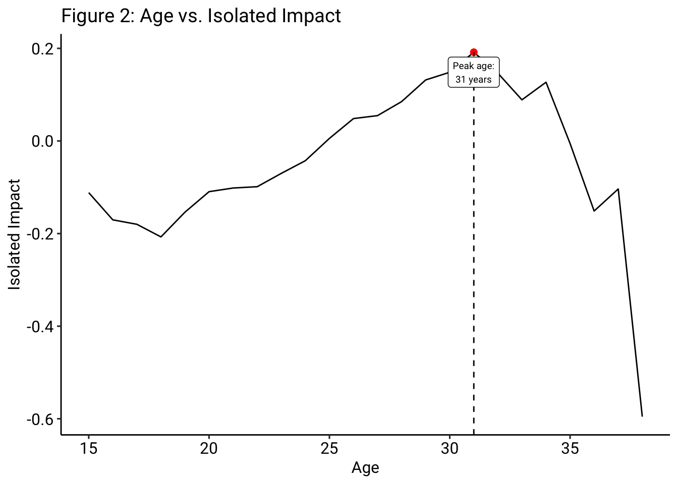
Given that there are a number of excellent players that are 30+, Messi, Ronaldo, and Lewandowski all come to mind, the baseline ability level of the remaining players over 30 years of age in the data set may be skewing the results of the aging curve. As a result, in this case, based off of our priors regarding player aging, it seems as though the number of good players in their 30s are skewing the results. One thing to note here, though, is that all players do age in some way or another; even though there may be many excellent players over 30 years old, that does not mean that they haven’t started to decline, maybe even significantly. Some players, though, just have such a high level of baseline talent that their “decline” still leaves them better than pretty much everyone else, even if those other players are at their peak themselves.
When discussing survival bias in this context, it is crucial that we be precise about the multiple ways that this type of bias may materialize. First, as we alluded to above, there is survival bias due to the fact that the players included at the tails of the data set are, likely, much better than the average 18-year-old or 40-year-old footballers. This type of survival bias, though, can be mitigated by controlling for the ability of the players in our data set; incorporating player controls into the model, assuming that each player has a baseline level of ability, and strictly examining the change in their performance from season to season means that the extraordinary talent level of the players at the tails of the data set do not influence the results of the aging curve.
While this initial form of bias may have the largest magnitude, there are remaining forms of survival bias that do not relate to the “talent” level of players in the data set, but, rather, concern the different rates at which players in the sample may age as compared to those excluded from the sample. This latter type of survival bias is slightly more difficult to control for and the actual direction of this potential bias is ambiguous. Consider the following examples: players that age slowly following their peak may be more likely to play top-flight football for a longer period of time, which would cause our model to underestimate the impact of aging on performance decline. Similarly, players that are selected to play top-flight football at 18 years old may already be more developed than their age group peers, meaning that they have less room to improve as they age, which would cause our model to underestimate the impact of aging on performance improvement. Conversely, though, consider players that age extremely quickly following their peak, causing them to never play in the top 5 leagues again and, therefore, dropping out of the data set, even though they may have regressed to the mean if given another season to play. These players would cause the model to overestimate the impact of aging on performance decline. In addition, consider younger players that are given playing time with the expectation that they will significantly improve from season to season. As a result, this may cause the data set to only include young players that show large improvement from season to season, removing the young players that only modestly improve, causing the model to overestimate the impact of aging on performance improvement. As stated before, the total impact of these biases is ambiguous. Further, there have been attempts to control for these biases through the introduction of “phantom years,” but the impact of that strategy is not particularly encouraging.2
The Delta Method
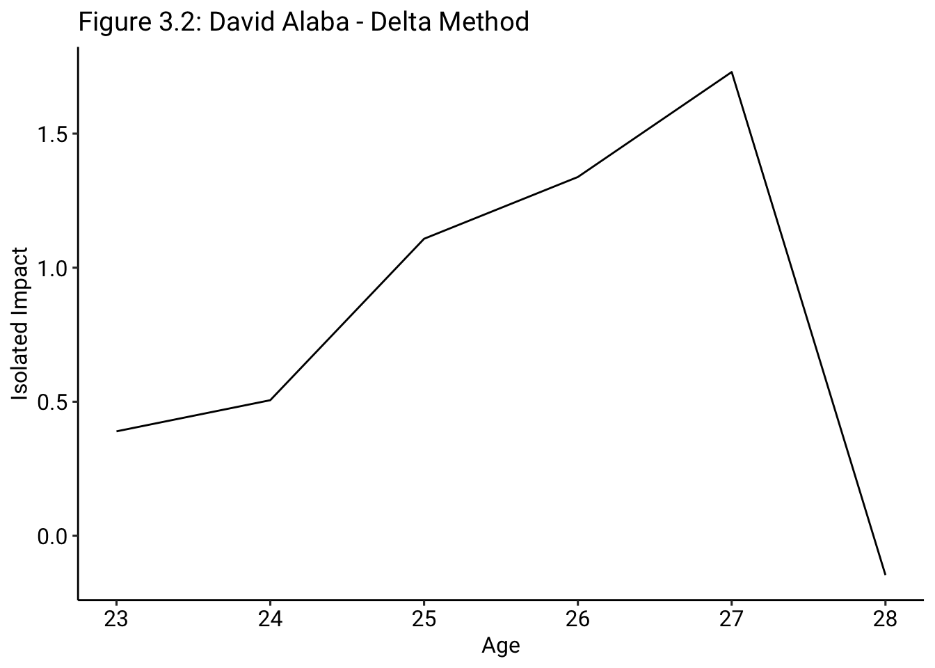
The second primary way that aging curves are calculated to assess player performance is through the “delta method,” a method that helps to mitigate survival bias, though it does pose a couple of additional, though more minor, problems. The delta method has been used in other sports, such as baseball, where the approach was pioneered by Tom Tango, and ice hockey, where Josh and Luke Younggren of EvolvingWild have written extensively on it. In addition, the delta method has been used previously in football analysis, where Michael Caley published additional research on aging curves. The delta method is calculated as follows: calculate the change, the “delta,” in the outcome variable of interest that occurred in two consecutive seasons and then, for each age bucket, such as 25 to 26, calculate the average delta value. For example, for David Alaba’s consecutive seasons ending in 2017 and 2018, we calculate the difference in Isolated Impact between the two seasons, which would be 5.53 - 4.92 = 0.61, as David Alaba’s “delta” for the age band of 24 to 25.
\(~\)
| Figure 3.1: David Alaba - Delta Method | |||||
|---|---|---|---|---|---|
| Age | Age Band |
Previous Season Isolated Impact |
Current Season Isolated Impact |
Delta | Cumulative Sum |
| 23 | 22/23 | 4.47 | 4.85 | 0.39 | 0.39 |
| 24 | 23/24 | 4.85 | 4.97 | 0.12 | 0.51 |
| 25 | 24/25 | 4.97 | 5.57 | 0.60 | 1.11 |
| 26 | 25/26 | 5.57 | 5.80 | 0.23 | 1.34 |
| 27 | 26/27 | 5.80 | 6.19 | 0.39 | 1.73 |
| 28 | 27/28 | 6.19 | 4.32 | -1.88 | -0.15 |
\(~\)
Then, to construct David Alaba’s individual “aging curve”, we simply have to calculate the cumulative sum of the individual age band deltas. In the example of David Alaba, as you can see, given the large negative delta between Alaba’s 27-year-old and 28-year-old seasons, it appears that his “peak” may have occurred at 27.3
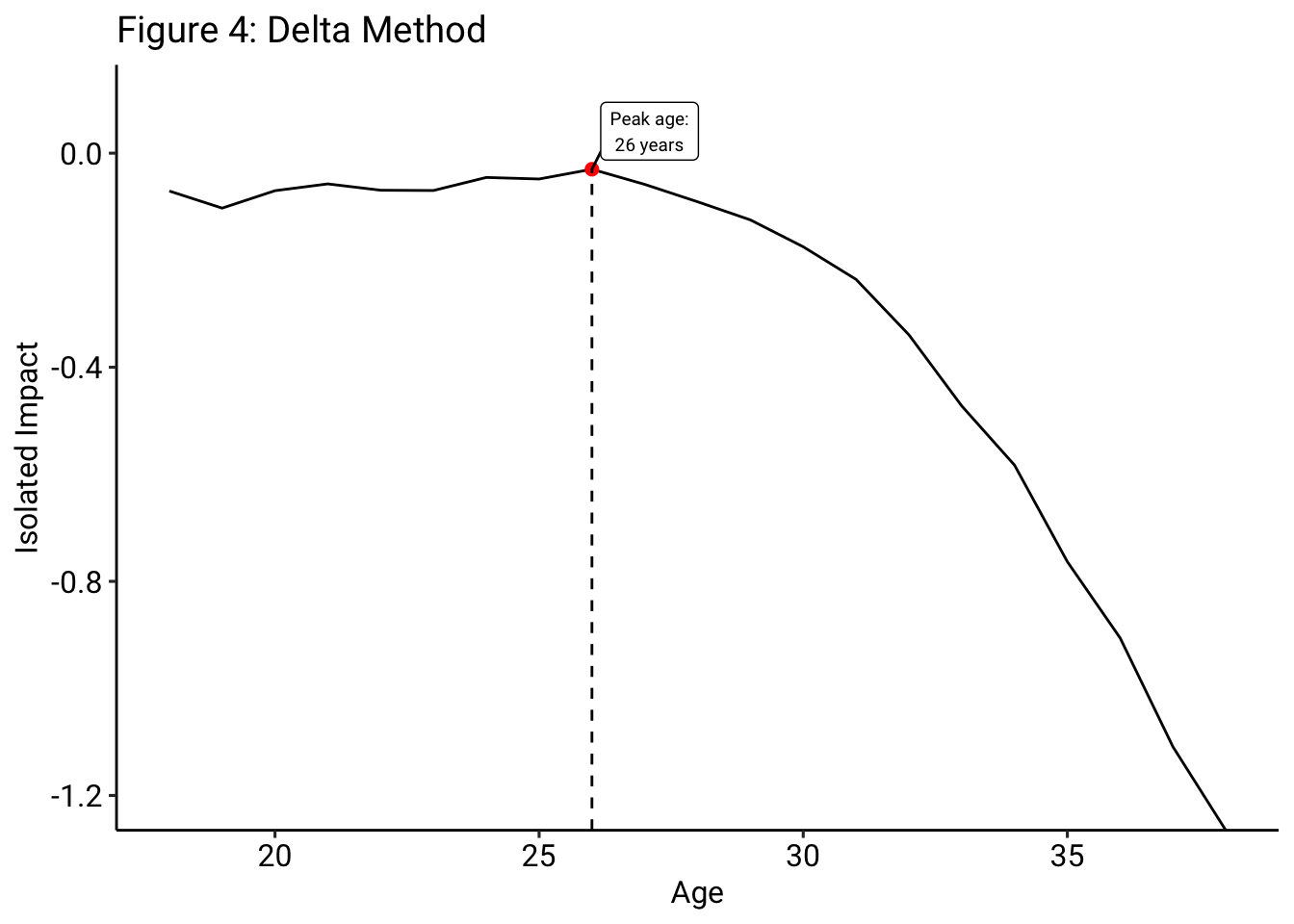
To construct the overall aging curve from this, the average “deltas” for each age band are calculated and then cumulatively summed. As we can see in Figure 4, the “peak” age, according to the delta method, is closer to 26, which is more in keeping with our priors and suggests that the delta method is, perhaps, mitigating much of the survivor bias that we noticed in Figure 2. How does the delta method, specifically, mitigate the issue of survival bias? It does so by controlling for player ability, meaning that the values of interest in construction of the curve are not the magnitudes of the variable of interest, but, rather, are the changes in the variable of interest, meaning that a player’s baseline level of ability has no influence on the shape of the curve; only the change in that ability from year to year has any influence on the shape of the curve.
But, while the delta method may help to mitigate some amount of bias, this methodology does, still, have several limitations, particularly as it pertains to our data set. First, it does not necessarily use a player’s entire career in the formulation of the player “talent” control; in order to accurately assess the impact of aging on footballer ability, player “talent,” or a player’s baseline ability, needs to be controlled for. In the delta method, given that the change in the outcome variable is strictly compared to the previous season’s value, the estimate of a player’s “talent” is only based on the outcome value from the previous season, rather than the player’s entire career. Second, the delta method severely restricts our sample size because only consecutive seasons can be used in the formulation of the aging curve. For example, if a player was in the European top 5 leagues during the 2015/16 season, but was not in the European top 5 leagues during the 2016/17 season, either due to relegation or a transfer to a different league, and then returned to the European top 5 leagues during the 2017/18 season, then the change in ability from 2015/16 to 2017/18 would be excluded from the delta method estimate. Given the frequency of relegation and transference to and from other leagues, the delta method causes a substantial number of observations to be excluded.4
Regression Method
To address the lingering issues posed by the delta method, while also continuing to control for player ability, we can use the third primary methodology to construct aging curves: regression. Regressions have been used in other sports, such as baseball, to estimate player “peaks”: JC Bradbury’s “Peak athletic performance and ageing: evidence from baseball” was one of the first articles to apply this technique. A regression is, at a basic level, an estimation of the relation between an outcome variable and one or more predictor variables. In this case, we are interested in determining the relationship between our outcome variable, Isolated Impact, and age, the predictor variable of interest. Rather than simply regressing Isolated Impact on age, though, we also need to control for player ability, as the delta method attempts to do by comparing the outcome variable with the previous year’s outcome variable value. As a result, we will use a regression model of the following form:
\[Isolated\,Impact \sim player + f(age)\]
In this model, \(player\) signifies the inclusion of a dummy variable for each player in the data set and \(f(age)\) is the function of age included in the model. Regression models, in comparison to the delta method, allow us to control for a player’s ability in a more robust fashion and include non-consecutive seasons. First, with regards to player ability controls, while the delta method only controls for “ability” as measured in the player’s prior season, this regression model controls for their player ability over the course of the player’s career. Second, the regression model can use all of a player’s observations within the data set, no matter the discontinuities in their careers.
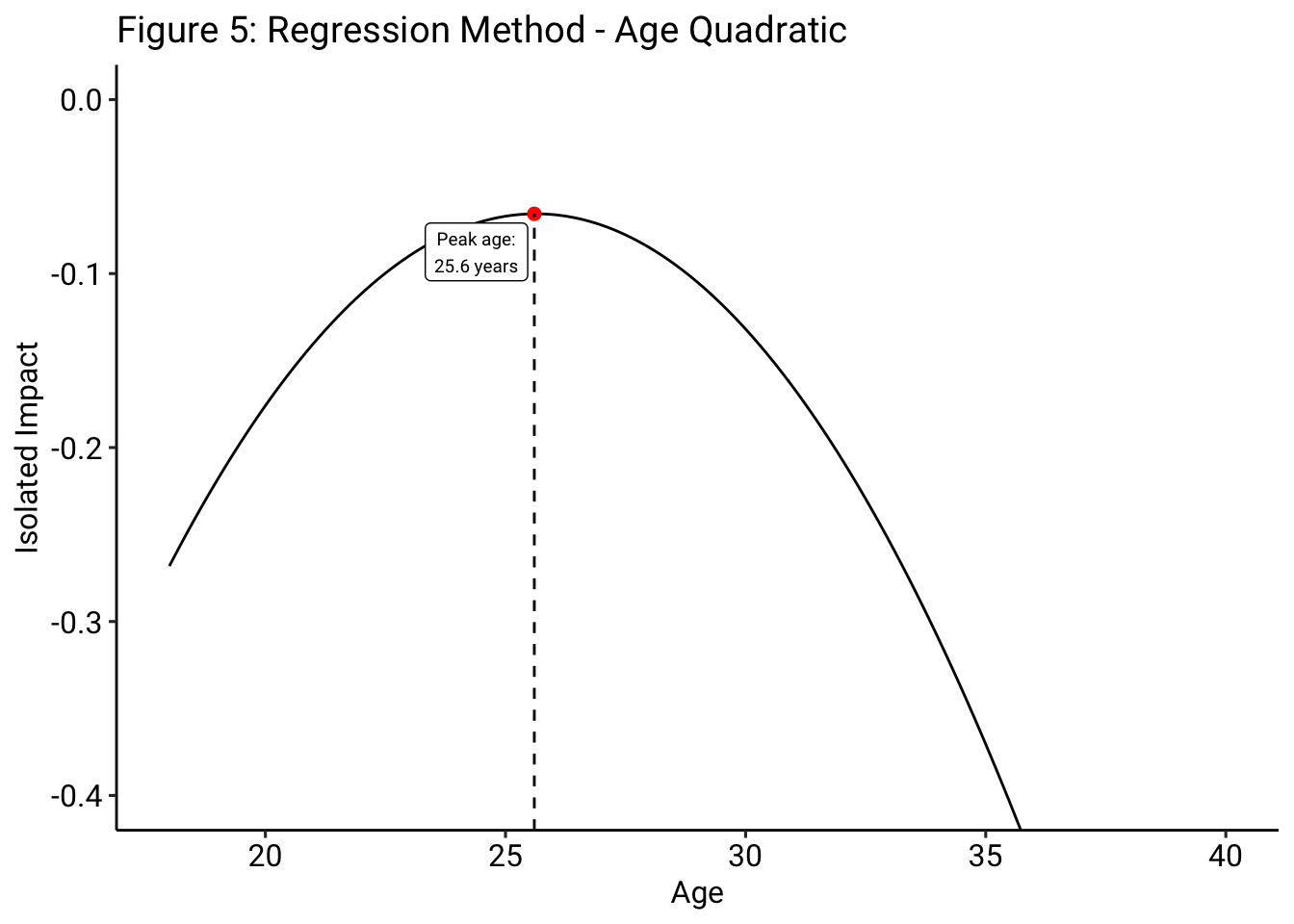
In order to effectively use the regression model, though, we must define the function of age that we wish to employ in the model. A basic regression methodology may use a simple quadratic function, where \(f(age) = \beta_{1}(age)^2 + \beta_{2}(age)\), which requires us to make various assumptions about how age affects player performance. Specifically, it requires us to assume that players improve at the same rate with which they decline, which could be true, but is, ultimately, unknown to us at this point.
3) Generalized Additive Model
Given that we do not want to have to make any sort of assumptions about the specific \(f(age)\) function, we can, instead, use a Generalized Additive Model (GAM). In a basic linear regression, an equation such as \(y = \beta_0 + \beta_1{x}\) is used to fit the data. In our aforementioned quadratic regression, the equation \(y = \beta_0 + \beta_1{(age)} + \beta_2{(age)^2}\), with player dummy variables omitted for simplicity, is used to fit the data. In a GAM, which is simply a generalized model where the impact of the predictor variables on the outcome variables are captured through smooth, non-parametric functions, meaning that the smooth functions can be either linear or nonlinear, the the shape of the predictor functions, the smooth functions, are determined by the data itself. In this case, once again omitting the player control variables for clarity, the GAM is defined as \(y = \beta_0 + s(x)\), where the previously mentioned function of x, \(f(x)\), is simply equal to a smooth, non-parametric function, \(s(x)\). Without going too deep into the weeds, we are actually going to be using a “spline” as our function for \(s(x)\), where a spline is a piece-wise polynomial curve. But, rather than presenting a series of disjointed piece-wise polynomials, the GAM smooths the piece-wise function into a continuous curve.5
To summarize, we are using a model of the form \(Isolated\,Impact \sim player + s(age)\) in order to estimate the impact of aging on player performance. Due to the inclusion of player controls, I want to note that the shape of the following player curves are not directly related to the ability level of a given player: the predicted aging curves, resulting from the GAM model, for Robert Lewandowski and Roberto Soldado will follow the same shape, though one of the curves will be located at a point higher on the y-axis because one of the players has a higher level of baseline “ability.”
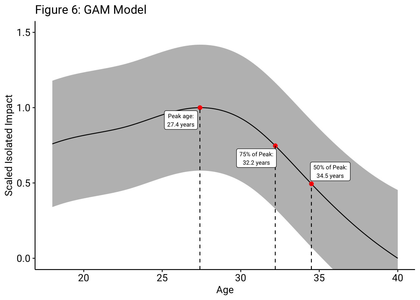
As shown in Figure 6, which fits the GAM model on the entirety of the data set, I find that footballers in the top 5 European leagues reach their peak at 27.4 years of age. Further, because we are not only interested in the precise age that players peak, but also the pace at which players decline, we find that, following their peak, footballers regress to 75% of their peak, relative to their minimum value at the age of 40, at age 32.2. Further, we find that footballers regress to 50% of their peak, relative to their minimum value at 40, at age 34.5, meaning that players typically regress by half of a standard deviation by their mid-thirties.
As a note, the y-axis for the age curves throughout the remainder of this article are scaled such that the minimum value for a given curve is 0 and the maximum value for a given curve, the “peak”, is 1. To give a general sense of magnitude, a change from 1 to 0, from maximum to minimum, is generally equal to a change of 1 standard deviation in Isolated Impact. So, according to these aging curves, generally, a player going from their peak to their minimum has regressed about 1 standard deviation in Isolated Impact value.
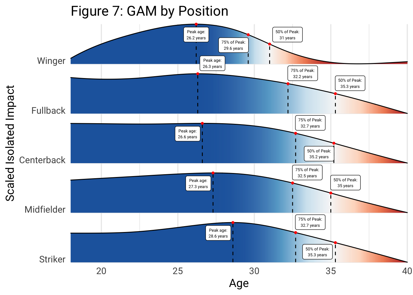
While it is interesting to be able to pinpoint, generally, when players peak and decline, there is likely significant heterogeneity in the impact of aging on player performance among different position groups. For example, we have heard plenty of times that wingers typically rely on quick changes of pace and speed in order to excel, while centerbacks can play at a high level without being quick or racking up lots of distance on the pitch. As a result, it would make sense if wingers aged relatively quickly, because once their pace declines they become significantly less useful, while centerbacks aged relatively slowly, because they can continue to play at a high level even without tremendous pace or agility. Figure 7, therefore, shows the aging curves segmented by position. In order to construct this, the GAM model is iterated over five unique data sets, one data set for each position, meaning that the aging curves for each position are independent from each other.
Figure 7 illustrates that, relatively in line with our priors, fullbacks and wingers, two positions that are traditionally reliant on pace, peak relatively early, around 26 years of age, centerbacks and midfielders peak at about 26.5 to 27.5 years of age, and strikers peak at about 28.5 years of age. Perhaps more interesting than their peaks is the fact that there is significant heterogeneity in the pace with which players decline from their peak across the different position groups. Once again in line with our priors, centerbacks take a long amount of time to decline: centerbacks decline to 50% of their peak, relative to their minimum value at 40, at 35.2 years old. Wingers, conversely, decline to 50% of their peak at 31 years old.
An interesting thing to note here is that the aging curve for wingers is the only curve where the value at 18 years old is anywhere close to the curve’s minimum value at age 40. My primary theory for this relates to the second, lingering, category of survivor bias that we discussed previously: wingers, generally, get to play football in the top 5 European leagues earlier than players in other positions. The preference to play more young wingers than young players at any other position indicates that more “raw” wingers may be allowed to play first team football at a young age. For all other positions, only the best, most talented 18-year-olds get to play in the top 5 European leagues. These players are, likely, already very developed (they must have been in order to stand out against their peers). As a result, the 18-year-olds included in the sample for non-winger positions do not have much room to grow and, as a result, the data is getting skewed such that those position’s peaks are only about 25% higher than their ability level at 18. In contrast, for wingers, there are a slew of 18-year-olds getting playing time that may not really be ready for top flight football and still have ample room to grow.6 In the final section of this paper, I propose a solution to help remedy this problem.
4) GAM and Tensor
In the first section of this paper, we introduced the three major overarching methodologies that have been employed to estimate the impact of aging. In the second section of this paper, we built upon the regression methodology by using a GAM to more flexibly estimate the relationship between age and performance. Further, we iterated the model over position-specific data sets in order to capture some of the heterogeneity in aging across position groups.
But, there are still two problems with our basic GAM model. First, we know that individual players age at different rates from each other: we will attempt to quantify this range of individual aging curves. Second, when aggregating at the position level, we know that segmenting the data by position and then iterating over those position-specific data sets may be suffering from position-specific forms of survivor bias: we will attempt to mitigate this specific bias by fitting all of the data with a single GAM, while using a variable to control for position-specific trend differences.
In order to quantify the different rates at which individual players may age, I include an additional variable, noted as the “decay rate” by CJ Turturo, for each player, which functions to slightly alter the overarching aging curve in order to better fit the individual player’s trend. As CJ formulates, “each player has [a] set of points for their performance in every season they’ve played, relative to their age at the time of that performance.” Further, he notes that, according to work done by JC Bradbury, the shape of the curve of a player’s performance relative to their age, would likely follow a quadratic pattern. Therefore, in order to measure each individual player’s unique aging progression, we fit the following quadratic curve, \(f(x)=ax^2+bx+c\), to every player in the data set. Then, given that the coefficient \(a\) of the quadratic is the coefficient that adjusts the steepness of the parabola, we define that coefficient \(a\) for each player as the player’s individual “decay rate.” Therefore, we now have a third predictor variable for our model: as before, we have individual player dummy variables, which control for the “ability” of a player, we have a variable for the general impact of aging, and we, now, have a variable that adjusts the aging trend to the specific player’s “decay rate.” Unlike before, in our original GAM models, we will not be using \(s(age)\), but, rather, will be using a tool that allows the individual decay rates to impact the overall impact of aging.
Specifically, we are going to be using a tensor product, which is a function that GAMs can utilize in order to incorporate interactions between predictor variables on different scales. In our case, the two predictor variables are \(age\), measured in years, and \(decay\,rate\), measured in Isolated Impact standard deviations. The model, then, that we will use to estimate how individual players age is as follows:
\[Isolated\,Impact \sim player + te(age,decay)\]
Obviously, with a third dimension of interest added to the model, we have to be more precise in defining what we want to visualize. As mentioned before, we know that assessing how age impacts performance requires individual inquiry. We are, therefore, using the “decay rate” variable to build that aging heterogeneity into the model. So, the purpose of using this individual player decay rate variable is to more formally characterize the range of likely aging curves for individual players. As a result, we are going to attempt to visualize the range of typical individual aging curves by grouping the individual decay rates into 10 quantiles and then plotting the aging curve for the minimum decay rate value for each quantile.7 As we can see in Figure 8.1, the majority of individual aging curves have a peak ranging from 26.5 years to 28.5 years old. But, Figure 8.1 shows that some players peak much younger, around 25 years old, and, in fact, some players may actually peak as early as 18 years old, implying that “young” players do not, ubiquitously, improve throughout their early 20s.
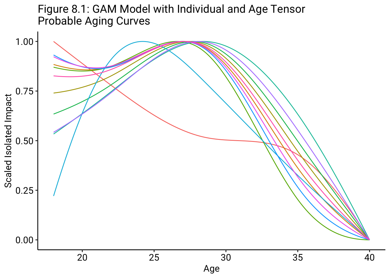
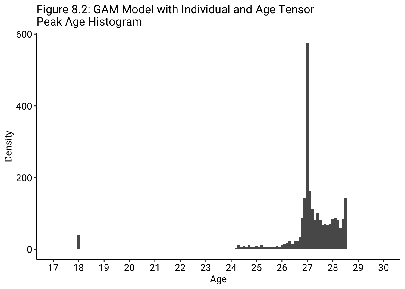
Figure 8.2 shows the distribution of player peaks according to the GAM model with the individual player decay rate and age tensor. As we can see, the majority of players peak, according to this model specification, from 26 years of age to 29 years of age. To provide a specific example, according to this model, Kevin De Bruyne, who is currently 30 years old, “peaked” when he was about 27.5 years old.
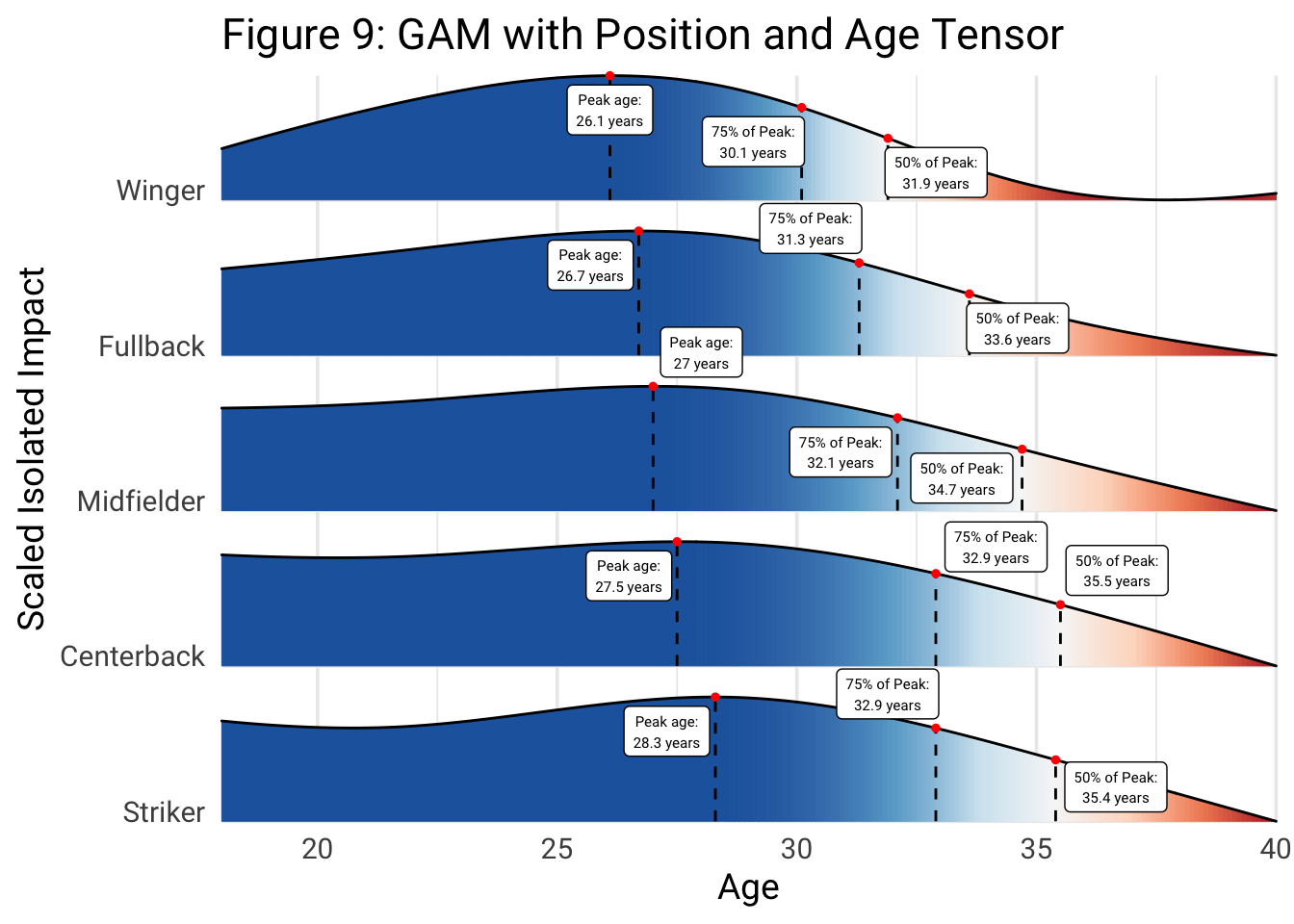
In the final model of this paper, we are going to try to improve upon our characterization of age impacts by position. Rather than splitting up the data into independent training sets according to position, by using a tensor with age and a unique “decay rate” variable for each position group, the model can tune the overall aging curve, while, simultaneously, using the individual position “decay rates” to inform the predicted aging curve for different position groups. Specifically, we will be using the same model used in the construction of Figure 8.1 and 8.2, but, rather than using decay rates specific to each player in the data set, we will use a single decay rate for each of the five position groups.
As a result, while the positional aging curves using distinct data sets suffered from the limited samples available for certain ages in certain positions, the positional tensor model can leverage, for all of the positions in the data set, the entire data set in the construction of the aging curve. Therefore, as we can see in Figure 9, the aging curve for wingers, when incorporating the full data set by using a positional tensor, does not indicate that wingers are better at age 32.5 than they are at age 18. We do, though, once again find that wingers and fullbacks peak the earliest, around 26 to 27 years old. Midfielders, according to this specification, also peak around 27 years old, while centerbacks and strikers peak around 27.5 to 28 years old. Once again, similarly to the previous model, for players in their 30s, centerbacks are typically closer to their peak than players in other positions; in other words, this model supports the idea that centerbacks in their 30s, generally, have declined less than players in other positions. In addition, while the model does suggest that wingers, generally, decline at an early age, the model does, conversely, suggest that 18-year-old wingers are only at about 50% of their peak, meaning that, by age 26, when they peak, they will be about 0.5 standard deviations better in terms of Isolated Impact. Other positions, on the other hand, are typically at about 70 to 85% of their peak at 18 years old, indicating that they might not actually have as much room to improve as has typically been assumed.8
Once again, though, this finding regarding improvement is really only applicable to 18-year-olds that are playing in Europe’s top 5 leagues. What I mean by this is that an 18-year-old academy player that hasn’t played a minute for the first team may improve far more than this aging curve implies. Specifically, this aging curve is built upon the career trajectories of players that are good enough to play top flight football; 18-year-olds that are not good enough to play top flight football may, actually, age at a different rate than players that are good enough.
5) Limitations
As mentioned throughout, there is one main limitation that persists throughout the GAM model specifications. While the regression model approach to the construction of aging curves helps to deal with the primary form of survival bias by controlling for player ability, there is still the possibility of a more minor form of survival bias that could persist: as mentioned previously, if the players towards the tails of the distribution, for example, the 18-year-olds and 40-year-olds, are systematically affected by age differently than those not included in the data set, meaning that they age at different rates than those excluded from the data set, then this would bias the results, though the direction of the possible bias is ambiguous.
Finally, while I believe that categorizing players by position can help to identify how aging heterogeneously affects different types of players, positions themselves are not the most accurate proxy for grouping players according to the varying roles they play in matches. Specifically, rather than grouping players by position, it is likely more informative to group player’s by their role (ie. box-to-box midfielders, deep-lying playmakers, and ball-winning midfielders may all age differently due to the requirements of their respective roles). Perhaps, I will generate a part 2 to this paper that analyzes aging by player role, rather than position.
6) Conclusion
Ultimately, as I have shown above, football players in Europe’s top 5 leagues, on average, “peak” at 27.4 years of age. In addition, when incorporating the individual heterogeneity in aging with the decay rate and age tensor variable, we find that football players, generally, peak between 26 and 29 years of age. Further, we find that there is heterogeneity in aging among players in different positions: wingers and fullbacks both tend to peak early, around 26 to 27 years of age, though wingers decline much faster than fullbacks. Midfielders also tend to peak at around 27 years of age, while centerbacks and strikers tend to peak around 27.5 to 28 years of age. In addition, centerbacks tend to remain closer to their peak later into their 30s. While individual inquiry is, obviously, still necessary, this approach to evaluating aging attempts to incorporate some of that heterogeneity into the model, while, simultaneously, using an outcome variable, Isolated Impact, that can be used to evaluate player performance across all outfield positions.
I am not including any type of “shooting impact” variable in this analysis. While it may be of interest to determine how aging impacts finishing ability, number of shots taken, or raw xG totals, those statistics are not really of interest in assessing the performance of the majority of players on the pitch. Given that the goal of this analysis is to generate an understanding of aging across different positions, it does not seem prudent to use statistics that are only relevant to the performance of one or two positions. With that being said, though, while I do believe that “Isolated Impact” encapsulates much of the relevant “ability” for outfield players, I do not believe that it captures the relevant “ability” of goalkeepers, which, more than anything, is related to shot-stopping. As an unintended consequence, therefore, goalkeepers are not included in this analysis. A future area of research may be to compare the aging curves of shooters and shot-stoppers, using some form of shooting ability and shot stopping ability metrics.↩
CJ Turturo performed a robustness test that incorporated “phantom years” in Flexible Aging in the NHL Using GAM and found that it actually reduced model performance.↩
This “peak” does not mean that David Alaba is now bad. One of the merits of the “delta” method over the basic plot is that it focuses strictly on the changes from age to age of a given player and the player’s overall ability level does not matter.↩
In the raw data set of Isolated Impact scores for each player in each of Europe’s top 5 leagues from the 2014/15 through 2020/21 seasons, there are 15,591 unique player and season combinations: for example, Lionel Messi’s 2020/21 season counts as a single observation. When the data set is filtered for the delta method to only include an observation if the given player was in the top 5 European leagues for the season directly preceding or succeeding the given season (meaning that the player was in the top 5 European leagues in the season prior or following the season in the observation), only 9,774 player and season combinations remain. This means that the delta method, in this basic implementation, reduces the data set by about a third.↩
GAMs offer various options for the “smooth” terms: I found that the P-splines, proposed by Eilers and Marx (1996) in “Flexible Smoothing with B-splines and Penalties”, when applied to this data set, produced the lowest AIC as compared to the other “smooth” term options.↩
In the 7 seasons of data included in this research, the 2014/15 through 2020/21 seasons, 11.6% of wingers have a season in the data set where they were playing in Europe’s top 5 leagues at age 18. In contrast, only 5.7% of centerbacks have a season in the data set where they were playing in Europe’s top 5 leagues at age 18.↩
Note that for the 10th quantile, the aging curve for the maximum decay rate value is plotted as well↩
I want to reiterate here that Isolated Impact is a per 90 statistic, meaning that 18-year-olds may get much more playing time as they age, but that would not directly improve their Isolated Impact value.↩